
I have a simplified approach in analyzing fish population dynamics from which I review the status of populations of smelt and salmon. It looks at the dynamics of the relationship between the number of spawning adults and their returning adult recruits one to several years later (Figure 1). In the fish science vernacular, it is sometimes referred to as the “spawner-recruit curve” or “stock-recruitment relationship” or simply “S/R relationship”. The major features of a S/R relationship are shown in Figure 1 (A, B, and C):
A. The blue and red curves show a standard spawner-recruit relationship, with higher spawners bringing more recruits – more eggs, more young, more smolts, more returning spawners, etc. It tails off when too many adults result in competition for food or spawning habitat, or higher rates of communicable disease – density-dependent effects.
B. The variability around the blue and red curves, shown by the vertical lines through the curves, is caused by density-independent effects such as drought, fishing harvest, or pollution that vary from year to year.
C. The difference between the blue and red curves, shown in the example as a yellow arrow, is a shift in the S/R curve that is a result in a fundamental shift in the relationship. Examples of such changes are the amount or quality of habitat from a dam being built, watershed destruction from a fire, loss of streamflow from new water diversions, loss of prey base, etc. The blue curve shows the S/R relationship before a fundamental shift; the red curve shows the S/R relationship after the fundamental shift.
Some environmental factors can affect one or more of the three features. For example, hatcheries can increase recruits (A and B), or they can cause a fundamental shift in the relationship (C) by imposing genetic changes in the population. Hatcheries benefit egg viability and fry survival, producing more smolts to the ocean per spawner in salmon populations, but may alter the wild component’s genetic viability.
The winter-run salmon population’s S/R relationship (Figure 2) exhibits these features, as well as the overall complexity in the relationship. Hatchery smolt introductions have propped up the population over the past two decades and increased its variability (red curve and vertical line), especially during periods of drought.
For longfin smelt, a state-listed species, there is a strong S/R relationship (Figure 3) to the features described in A-C above. There is a strong positive S/R relationship (A). There is a strong effect of the climate (B). And there appears to be a fundamental shift in recent years (C).
For Delta smelt (Figure 4), a state- and federally-listed species, which I consider nearly extinct at least in the wild, there was a strong S/R relationship (A), a climate effect (B), and a fundamental shift (C). The latter proved simply not sustainable, leading to a population crash that is not recoverable without supplementation (hatchery inputs) or drastic changes In environmental conditions.1 Note that 2016 is the last year in this figure, because the population since 2017 has been too close to zero to evaluate.
The largest salmon population, the Sacramento fall-run salmon, long sustained by hatchery inputs, is mainly controlled by feature B (Figure 5). Climate and water management are the dominant control of survival of hatchery and naturally-produced smolts reaching the ocean.
In conclusion, I recognize that S/R relationships represent a simplified view of extremely complex and changing relationships in the real world. Estimates of the number of spawners and recruits are often crude. But the relationships are real and statistically significant. It is up to us to interpret them by relating causal factors and developing hypotheses that can be tested with further scientific study and experiments. Unfortunately, managing fishery resources in the face of complex ecology, difficulty monitoring, natural variability, and statistical measurement errors is inherently difficult, even before political and economic factors get into the mix.
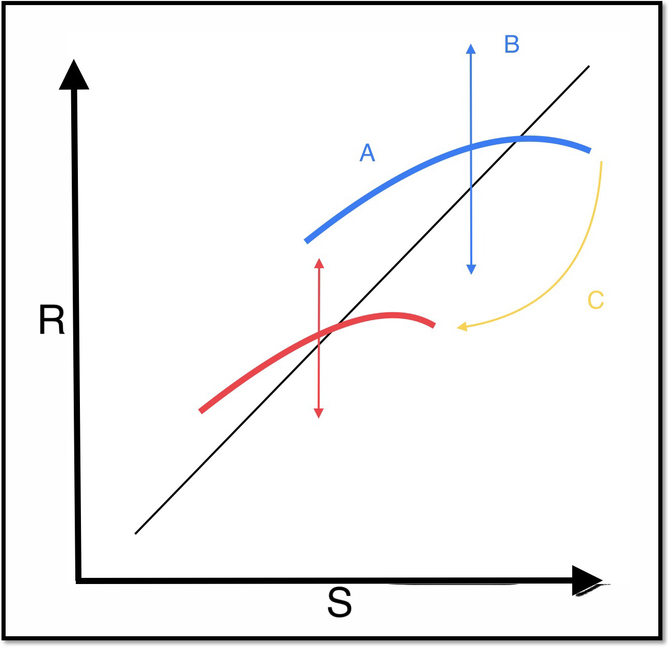
Figure 1. Spawner-Recruit relationships with three main features (A-C). See text for explanation of the features. In figures 2-4 below, the blue curve represents the historical S/R relationship. The red curve represents the new historical S/R relationship following a fundamental shift in the relationship, including long-term drought. The vertical lines through the curves show the range of the annual variability of the S/R relationship attached to each curve, excluding the density-dependent variability that is incorporated into the curve. In this example figure, the yellow curve tracks a fundamental shift in the S/R relationship. Spawners are shown on the x-axis; recruits are shown on the y-axis. The numbers on the axes are log transformed in order to make size of the figures manageable; log transformation does not alter the statistical relationships.
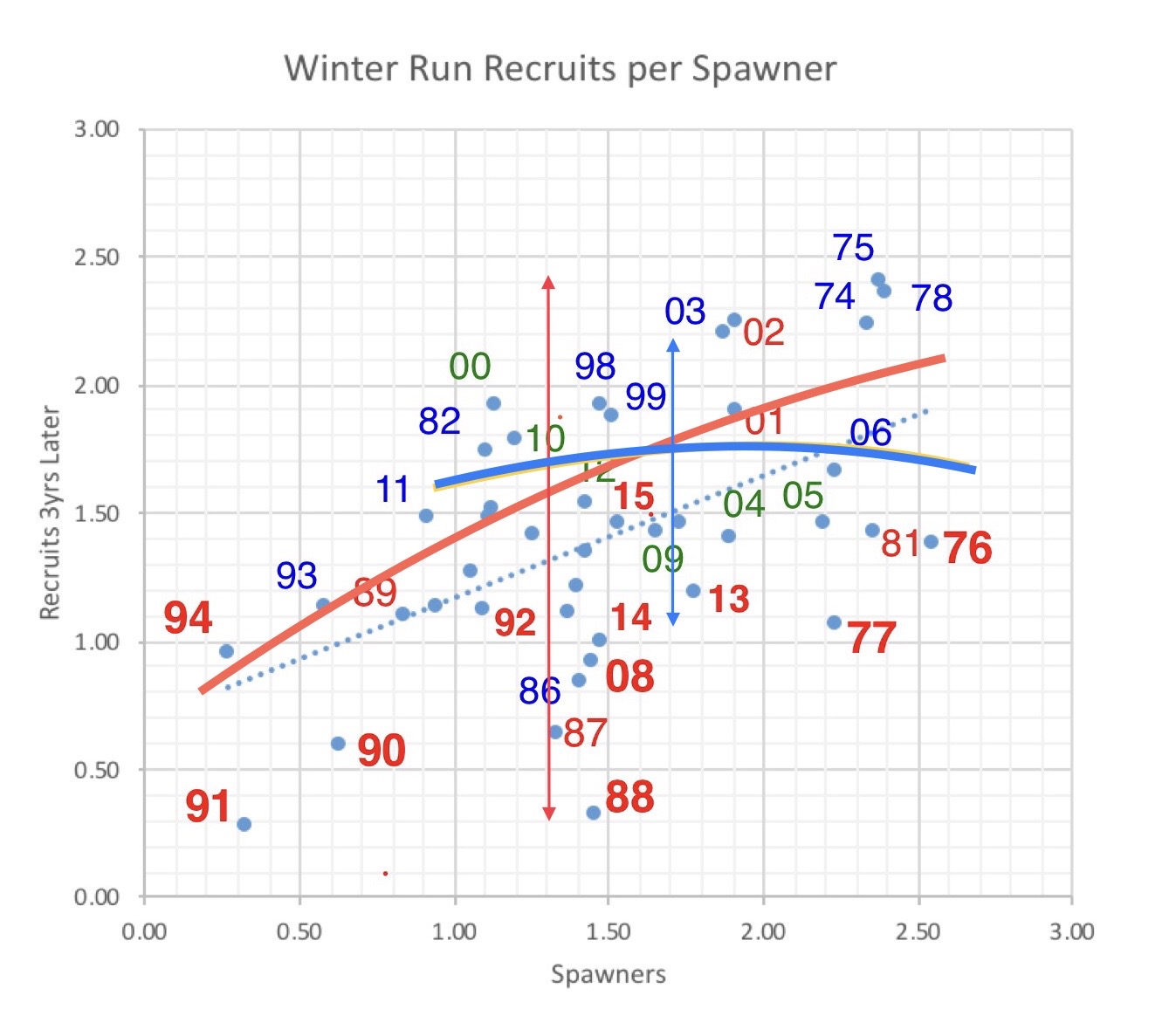
Figure 2. Spawner-Recruit relationship for winter-run Chinook salmon in the Sacramento River. Numbers shown represent the brood year of recruits (number of returning adults) for year displayed. For example, “11” represents fish produced in wet year 2011. The color of the number shows the conditions when brood was spawned and reared in the upper Sacramento River below Shasta Dam before emigrating to the ocean. A red number shows a dry year during spawning and early rearing. A blue number designates wet year spawning and rearing conditions. A green number designates normal water year conditions. For example, 15 represents brood-year 2015 recruits that returned in 2018, while its red color designates drought conditions in 2015. In this figure, numbers on axes are log-2 transformed.
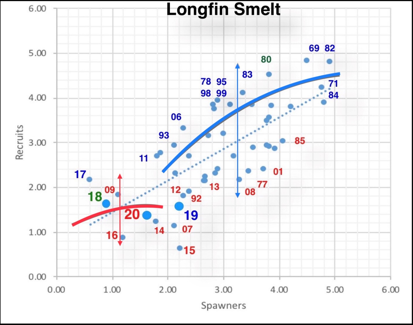
Figure 3. The longfin smelt S/R relationship. The number and color represents the brood year’s fall index (recruits) and its water year type during its spawning run and first year of rearing. The spawners are the index from two years earlier. For example, the red number 15 represents the fall index for brood-year 2015 under water-year 2015 drought conditions, with spawners being the recruits from 2013. In this figure, numbers on axes are log-log transformed.
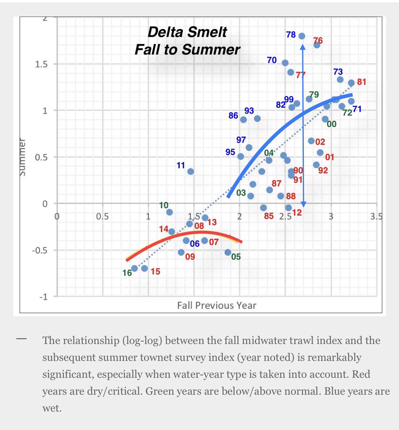
Figure 4. The Delta Smelt S/R relationship. I added two curves and a vertical line to an original figure to show the hypothesized S/R relationship; there is too little variability in the red curve for a vertical line to be meaningful.
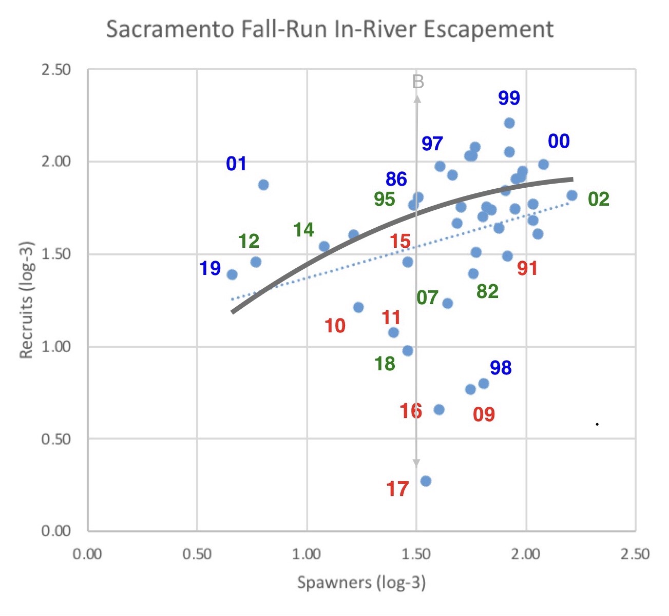
Figure 5. Spawner-Recruit relationship for upper Sacramento River mainstem fall-run Chinook salmon. Number is recruitment year (escapement). Spawners are recruits from three years prior. Numbers are log minus 3 transformed. A red number shows a dry water year two years prior during rearing and emigration. A blue number shows a wet year two years prior. A green number shows for a normal water year two years prior. For example: red 17 represents 2017 run that reared in drought year 2015, with spawners (parents) being the 2014 green run number. Note that only one curve is shown. in gray, for this run of salmon, which is almost entirely dependent on hatchery production.